1 Introduction
1.1 Double-slit experiment
We start by looking at one of the most famous quantum experiments to get an idea of the surprising nature of quantum behaviour.
In the double slit experiment, a light source is placed behind a wall with two narrow, closely spaced slits. On the other side, a photosensitive plate is positioned.

An interference pattern appears on this photo plate, i.e. alternating light and dark stripes. This is due to the wave character of light. As the light waves pass through the slits, they overlap and interfere with each other. In some areas they have the same amplitude and reinforce each other, creating bright stripes. In other areas, the amplitudes have different signs and the waves cancel each other out, creating dark stripes.
This behaviour is to be expected. This is because the light travels different distances from the two slits to the same spot on the photo plate. If the difference is half a wavelength the two light waves cancel out at that spot.
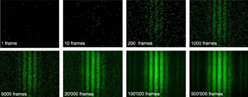
Now we take individual photons. Here we would expect the interference pattern to disappear, as each photon can only pass through one of the slits. In that case, no interference can occur between photons coming from the two slits since they never meet. We would expect just two overlapping bright areas.
Surprisingly this behaviour does not occur. Even with single photons an interference pattern continues to appear. The photons do not decide to pass through one specific slit. They are in “superposition” between these two paths. This means that a single photon has two possibilities where it came from, both possibilities still happen at the same time and can cause interference with each other. For this reason, the amplitudes also add up or cancel out at the photo plate, resulting in the same interference pattern.
In later chapters, the mathematics shown will make this behaviour easier to understand.
1.2 What is a quantum computer?
To start into the topic of quantum computing and to understand the differences from classical computers, we first need to look at some of the basics of such classical computers.
In a classical computer the information is stored in bits which can either be in the state \(0\) or the state \(1\). These bits can be manipulated through different classical operations and we can look at these bits and read them, without interfering with the system or changing any states.
In a quantum computer the information is stored in a qubit which can be in a superposition between the state \(0\) and \(1\). Just as with classical computers, we can construct variables from these qubits to store bigger numbers. For example a 64-qubit integer would be described by 64 qubits which are in a superposition between \(0\) and \(2^{64}-1\). This can be imagined best as a variable where the universe has not yet decided on its value and therefore the variable has all possible values at the same time.
We can now use this superposition and manipulate it with different quantum operations. Contrary to a classical computer, in a quantum computer these operations are “applied” at all possible input values at the same time and the result is a superposition of all possible results of the operation. We call this effect quantum parallelism.
Reading this, one might be tempted to utilize quantum parallelism to run any algorithm on a quantum computer in order to optimize runtime. Unfortunately there is a big catch with quantum computers: If we try to look at the state of a qubit (also called measuring), the universe decides randomly on an outcome and therefore when measuring we only get the result of one computation and all the rest of the information is lost.
Due to this restriction, naively running established algorithms on a quantum computer will not work. Fortunately there are some clever tricks to create some “interference” between different computations before measuring. This will give us useful information in some cases.